TL;DR: In this post, we will learn the basic concepts of linear graph signal processing and see how they’re related to classical signal processing. By the end of this post, you will understand what are graph signals, their relation to time domain signals, representation of graph signals in the vertex and the spectral domain, Graph Fourier transform and efficient spectral filtering.
Notice: Even though relevant material is mostly linked, basic background in Fourier-analysis, spectral-analysis and convolution theory may simplify the read.

Data appears in various shapes. Many data sources are obtained from raw natural scenes, such as in images, motion trajectories, video or sound, which are inherently unstructured and typically demonstrate continuities, smoothness, and regularity. These high-level constraints impose prior knowledge that can be utilized and formulated for modeling these signals. Other data sources include structured data types, such as tables and graphs, with discrete associations, irregular properties and relational structure. These structures may seem more complicated and harder to grasp, however, their unique organization is highly compact, very efficient and great for search. Typically, a graph’s connectome, or wiring network, holds rich information on its entities, and thus becomes an interesting subject in many different contexts. Formally, relational graph data is represented with $G=\{V,E,W_E\}$ where $V$ , $E$ and $W_E$ denote the group of vertexes (or nodes), edges (links or connections) and edge’s weight respectively. In order to make life a bit easier, the graphs in this discussion are undirected.

The first concept one should discuss in a GSP introduction would probably be - How do we define a signal over a graph? Intuitively, a signal $s$ on graph $G$ can be seen as a vector of scalars over the nodes, and formally

$s:V\rightarrow \mathbb{R}^N$

Graph-structured data enables to recruit both the network structure and the node’s properties (features) for solving difficult tasks. In Neuroscience, for example, the network connectivity structure can be inferred as a graph, with edges connecting distinct functional regions, when each region is characterized by its sensory association, location, area and response pattern to various stimuli. In this post, we will see that various tools and concepts from traditional signal processing can be applied to graph data, only if first we associate the graph’s architecture with the time-axis.

Simple graph signal example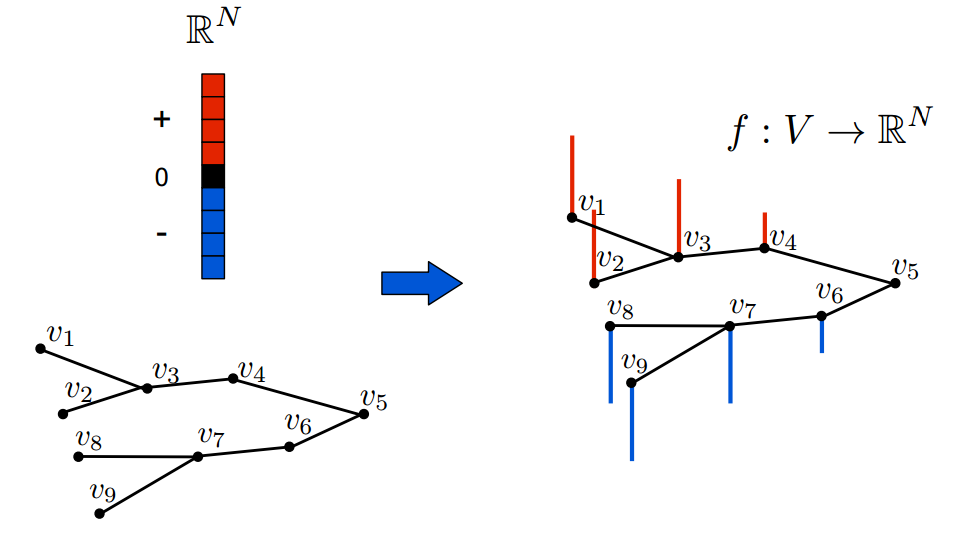

Background - The shift operator in Signal Processing

Digital Signal Processing (DSP) is typically referred to as manipulating single or multidimensional signals in either the time or spectral domain. Working with the spectral representation of signals has various advantages, such as effective sampling, simplified mathematical analysis (filtering for example), efficient and informative dimensionality and many more. Yet, in order to work in the spectral domain, we commonly need to apply some kind of transformation as the Fourier, Wavelet or Laplace transform. As a side note, DSP has strong connections to popular and trendy techniques, such as Deep learning, as the linear transformations that are applied on each layer of the network, are effectively linear filters that project the data to some learned and efficient “task” related domain.

A popular transform in DSP is the $z$ -transform¹ which essentially expands signal $s\in\mathbb{R}^{N\times 1}$ to a scaled power series, or a Laurent series

$Z(s[n])=\sum_{n=0}^{N-1}s_n z^{-n}$

The $z$ -transform is one of the fundamental building blocks of modern signal processing, when it’s the most basic polynomial term, i.e. $z^{-1}$ , is frequently referred as the signal’s time delay or shift. In order to gain some intuition for its name, let’s use the shift to filter the discrete Dirac’s delta function $\delta[n-k]$ , which is a fully flat signal of zero’s with 1 in the $k$ -th location. This is achieved by multiplying the $z$ -transformed version of $\delta[n]$ with the $z$ -transformed filter $h_{\text{shift}}[z]$ , which is also expressed as a power series of the shift

$Z(\delta[n])=\sum_{k=0}^{N-1}\delta[n-k] z^{-k}=1\cdot z^0+0\cdot z^{-1} +...=z^0=1$ $h_{\text{shift}}(z)=\sum_{n=0}^{N-1}h_n z^{-n}=1\cdot z^{-1}+0\cdot z^{-2}+...=z^{-1}$

Therefore, applying the filter would result in

$Z(\delta[n])\cdot h_{\text{shift}}(z)=z^0\cdot z^{-1}+0\cdot z^{-2} +0\cdot z^{-3} +...=z^{-1}=Z(\delta[n-1])$

It appears that this manipulation is actually shifting the signal by one sample. Accordingly, in order to enable linear filtering and to obtain a spectral representation of graph signals, we would like to have a ‘shift-for-graph’ operator with equivalent properties. Notice that choosing $z^{-n}=\frac{1}{\sqrt{N}}e^{-j\frac{2\pi}{N}kn}$ leads to the frequency representation of signal $s$ , and particularly the Discrete Fourier Transform (DFT) which we will mention later.

The shift operator in graphs

In order to define the GSP counterpart, we will start by shifting again a time-domain signal, but now we take a graph-oriented perspective. In this example we use a periodic time-series signal $s=[s_0,s_1,...,s_{N-1}]^T$ , which holds a graphical structure of a directed cyclic graph, where $s[n]=s[n+N]$ .

Graph structure of a periodic time-series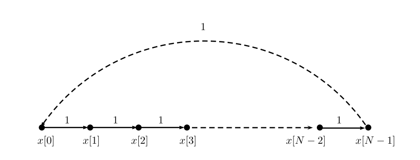

It appears, that the signal can be shifted by multiplying it with $A\in \mathbb{R}^{|V| \times |V|}$ , a cyclic shift matrix s.t. $s_{\text{shifted}}=A\cdot s$ when

$A = \begin{pmatrix} 0 & 0& ...& 1 \\ 1 & 0& ...& 0 \\ \vdots & \vdots& \ddots& \vdots \\ 0 & ...& 1& 0 \end{pmatrix}$

You may see that this cyclic graph operator is precisely the adjacency matrix of the above time-signal graph. The adjacency matrix is a symmetric matrix with entries equal to zero and one, when $a_{i,j}=0$ indicates that there is no link between node $i$ and node $j$ . In the time-domain signal, it defines the unidirectional information flow in the graph and supplies time-context to the set of graph-signal values. Notice that this linear operation is actually substituting the value of the node with its neighbor, or more generally - with a weighted sum of its neighbor’s values. This exemplifies an important property of the shift - it behaves as a local operator in the vertex domain. Other choices and variations for the graph shift matrix have been proposed, when popular choices are the non-normalized combinatorial graph Laplacian, $L=D-A$ and the symmetric normalized Laplacian, $\mathcal{L}=D^{-1/2}LD^{-1/2}$ , where $D$ is the degree matrix, a diagonal matrix with

$D_{i,j} = \left\{ \begin{array} {rcl} \sum_{j=1}^{|V|}a_{i,j} & \text{if} & i=j\\0 & \text{else} \end{array}\right.$

Similarly to the one-dimension Laplace operator, the graph Laplacian can be seen as a high-pass filter or difference between a signal on a node to the signals of its neighborhood. These alternative definitions for the shift remain weighted-sum local operators, when the answer to “Whom to select?” is not definite, as each option features particular trade-offs in terms of frequency representation (complex/real eigenvalues) and graph type compatibility (directed/undirected). A throughout analysis of the differences between $\mathcal{L}$ , $L$ and $A$ is presented in Lutzeyer & Walden, 2017. Further, novel alternatives for the shift operator, which preserve the energy content of the graph-signal, are suggested in Gavili & Zhang 2017, however, they are out of the scope of this post. For the rest of this blog, we will focus on the graph Laplacian $\mathcal{L}$ as the shift.

In conclusion:
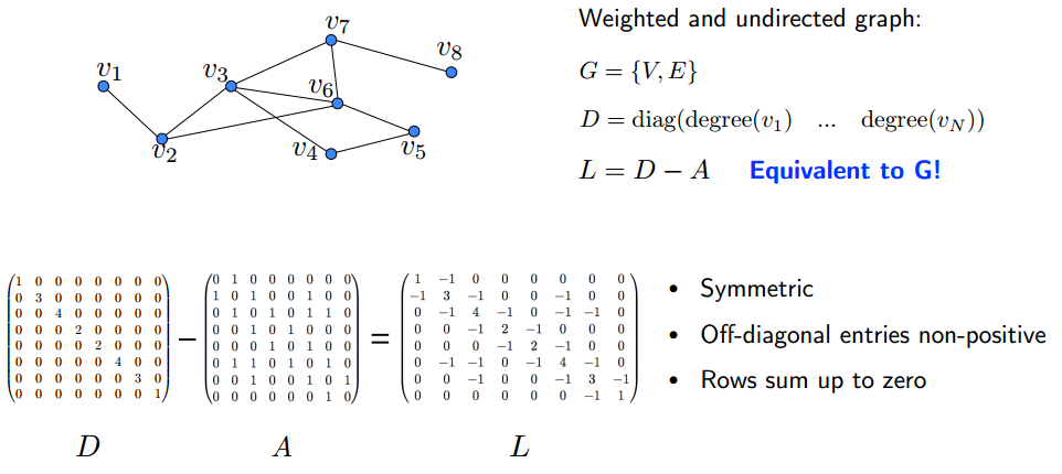
+ The $z$ -transform is a key representation for time and frequency analysis in classical DSP.
+ The most basic building block of this transformation is the shift, or time-delay, operation.
+ Some analogies for the shift in GSP are the graph adjacency matrix or different versions of the graph Laplacian.

Graph frequencies and the Graph Fourier Transform

Now that we understand the role of the shift in spectral representation and its definition in GSP, it is time to discuss the notion of graph frequencies. You may be already familiar with frequencies in time-domain, which are typically described as sinusoid oscillating at low to high rates. In GSP, low and high frequencies describe the amount of change between values of connected nodes in the graphs frequency components. The change itself is measured using graph total variation, which quantifies the normed total difference between a graph signal and its shifted version. In a micro view, this translates to the absolute difference between the node’s eigenvector value and his neighbors, s.t. the number of eigenvector’s zero-crossings indicate whether the frequency is low or high (see Sandryhaila & Moura 2014).

The graph frequency, or spectral components, are obtained via Spectral decomposition, where the graphical structure is decomposed into $n$ linearly-independent and distinct eigenvalues. One great advantage of this technique is that the estimated frequencies, or the graph spectrum, are totally invariant to node permutations. This is a highly desired property that defines an important constraint for graph learning tasks (see for example Simonovsky et al. 2018).In different from DSP, where the transform is not universal, as the network structure in the shift varies between graphs, and specific decomposition is needed for each graph format. For instance, the Laplacian shift $\mathcal{L}$ is a real symmetric matrix and therefore can be decomposed to the quadratic form

$\mathcal{L}=\chi\Lambda\chi^T$

where the columns of $\chi$ are the eigenvectors and $\Lambda$ is a diagonal matrix with $\lambda_i$ denoting the relative power of the $i$ -th eigenvector. Intuitively, eigenvector $\chi_i$ can be though as a Fourier’s basis function, $e^{j\omega x}$ , and $\lambda_i$ is the frequency of this function, when the lower the frequency is, the more regular or smooth the signal is.

Visual example of graph frequencies (Ortega and Dong slides)

In case you are familiar with the domain of spectral graph theory, you might recognize that the Rayleigh quotient is closely related to this decomposition. Specifically, if the eigenvectors, $\chi_i$ , are normalized, the minimum argument $\chi_i$ and its corresponding value $\lambda_i$ describe the quotient

$\lambda_i = \min_{\chi_i} \frac{\chi^T\mathcal{L}\chi}{\chi^T\chi}$

The Rayleigh quotient is a minimization task with various uses in several fields such as physics, mechanical elasticity, control theory, statistics and data science (see Bai et al. 2018). Personally, I was first introduced with the minimization problem when I studied Spectral clustering and the Graph Cut problem for image segmentation. In classical computer vision, this task was optimizing a binary vector which divided the Image Laplacian into two or more cuts, thereby separating the image to distinct segments (see Shi & Malik, 2000). The first nontrivial solution to this partition is the binarized Fiedler vector - the second eigenvalue of the quadratic form. Accordingly, spectral decomposition can be intuitively related to node clustering in graphical networks by observing low-pass frequencies.

As we already mentioned, the complex exponentials, which are the basis functions of the common Fourier transform (FT), are in fact the eigenfunctions of the one-dimensional Laplace operator, or alternatively the time-domain Laplacian (see code example). Accordingly, the eigenvectors of the graph Laplacian can be used to define the analogous Graph Fourier Transform of any signal $s$ over graph Laplacian $\mathcal{L}$

$\mathcal{F}_{\mathcal{L}}(s)=\chi^Ts=[\chi_1^Ts,\chi_2^Ts,...,\chi_{N-1}^Ts] \ \ \ \ \ \text{s.t.}\ \ \ \chi_i\mathcal{L}\chi_i^T=\lambda_i$

An explicit comparison of the Fourier Transform in time and graph domain, facilitates the analogy even more:

$\text{DSP - }\ \ \ \mathcal{F}_\omega(s)=\int(e^{j\omega t})^*s(t)dt\\\text{GSP - }\ \ \ \mathcal{F}_{\ell}(s)=\sum_i\chi_\ell^*(i)s(i)di$

when $\ell$ is analogous to the frequency term $\omega$ . Thus, the Fourier transform of $s$ can be abbreviated to $\mathcal{F}(s)=\chi^T s$

In conclusion:
+ The Fourier basis is the eigenbasis of the time-domain graph’s Laplacian.
+ High and low frequencies of graph signals translate to the number of zero-crossings in the graph spectral components.
+ Eigenvalue decomposition of the shift matrix leads to spectral components of the graph-signal.

Filtering graph signals - convolution in spectral and vertex domain

In this point, we have defined graph signals both in the frequency and the vertex domain. We also mentioned that frequency transformed time-series can be grasped as a linear combination of complex exponentials, where each coefficient denotes the amount of influence of the frequency component. Filtering is a basic task which allows to isolate the contribution of individual frequencies, and therefore enables to remove noise or observe dynamics in a specified spectrum. By defining the Graph Fourier Transform (GFT), we can use the famous Convolution Theorem to perform spectral filtering. In DSP, this theorem states that under suitable conditions “the Fourier transform of a convolution of two signals is the pointwise product of their Fourier transforms”. Recall that this principle was used in our early demonstration of filtering the Dirac’s delta signal with the shift. Accordingly, we can filter on input signal $s_{in}$ in the following manner

$s_{out}=H\cdot s_{in}=\chi h(\Lambda)\chi^T s_{in}\\=\chi \cdot \text{diag }\Big[h(\lambda_0),...,h(\lambda_{N-1})\Big]\cdot \hat{s_{in}}$

when the Fourier transform of $s_{in}$ is $\hat s_{in}=\chi^T s_{in}$ and $\chi$ is the inverse GFT. It is easier to identify the classic time-domain equations when looking on non-matrix notations

$\text{DSP - }\ \ \ \ s_{out}(t)=\int \hat s_{in}(\omega)\hat h(\omega)e^{j\omega t}=(s_{in}*h)(t) \\\text{GSP - }\ \ \ \ s_{out}(i)=\sum_{\ell=0}^{N-1} \hat s_{in}(\lambda_{\ell})\hat h(\lambda_{\ell})\chi_{\ell}(i) \qquad \qquad$

Obviously, this filtering method is expensive, as we need to calculate the eigen-decomposition of $\mathcal{L}$ . This diagonalization step has high computational cost and scales poorly in large networks. The problem can be relaxed by using polynomial filters, which do not require the GFT basis. With this filter we approximate the frequency response, $h(\lambda)$ as a linear combination of $K$ eigenvalues s.t.

$\hat h(\lambda_{\ell})\approx \sum^{K-1}_{k=0}a_k\lambda_{\ell}^k$

With little mathematical effort, one can describe the filtered signal on node $i$ with a power series of the shift matrix

$s_{out}(i)= \sum_{\ell=0}^{N-1} \hat s_{in}(\lambda_{\ell})\hat h(\lambda_{\ell})\chi_{\ell}(i) \\ =\sum_{j=1}^{N} s_{in}(j)\sum^K_{k=0}a_k\sum_{\ell=0}^{N-1} \lambda_{\ell}^k\chi^*_{\ell}(j)\chi_{\ell}(i) \\ =\sum_{j=1}^{N} s_{in}(j)\sum^{K-1}_{k=0}a_k (\mathcal{L}_{i,j})^k$

Effectively, we avoid the eigen-decomposition, and instead calculate the $K$ -th power of the shift for filtering the signal! Notice that this calculation uses the spectral decomposition of the Laplacian and the identity $\hat s_{in}=\chi^* s_{in}$ . Now let’s assume for a minute that instead of $\mathcal{L}$ we use the normalized adjacency matrix as the shift (normalizing by the degree of each node) and take a closer look on $(A_{i,j})^k$ .
It can be shown that $A_{i,j}$ denotes the probability of arriving in a 1-step random walk from node $i$ to node $j$ (see Lemma 5.2 in Hammond et al. 2009 ). When raised to the power of $k$ this term describes the following probability

$(A_{i,j})^k = \Pr(i_{\text{start}}\rightarrow j_{\text{end}}|\text{num steps}_{i\rightarrow j}=k)$

Particularly, this approximation enables us to encode the filtered signal on vertex $i$ , with structural information of its $K$ -hop environment, which introduces a nice interpretation of the filtering operation in the vertex domain.

Implementation via approximation

Polynomial approximation for localized graph filters are intended for saving computations, and specifically reduce the eigen-decomposition and multiplication. There are several popular approximations in GSP - Minmax, Meyer, Least Squares, Lanczos method and more, while the most popular approximation is known as the Chebysev expansion. We won’t dive deeply to its rigorous definition (maybe a future post), but only highlight that it is highly efficient due to the recursive formulation of the filter

$\hat h(\lambda_{\ell})\approx \sum^{K-1}_{k=0}a_kT_k(\tilde\Lambda) \quad \text{s.t.}\quad T_k(x)=2xT_{k-1}(x)-T_{k-2}(x)$

You can read more about the Chebyshev and other expansions in Hammond et al. ,2009 and Vandergheynst & Shuman, 2011

In conclusion:
+ The convolution theorem in DSP translates to practically a matrix product of the signal with the spectral components of the Laplacian.
+ Efficient implementation of graph filtering uses a power series of the Laplacian instead of eigen-decomposition.

Coding time!

Let’s practice GSP with python and pygsp

First example - The time-domain Laplacian and the Fourier transform

I will first demonstrate visually how the time-series analysis relates to GSP. Notice that plotting code is removed for brevity, but can be found in this gist.

First make sure that you’ve downloaded pygsp, which is a python implementation of the GSP Matlab package. It is very diverse and enables many operations, such as filtering, interpolating and plotting graph signals in the vertex and spectral domain. It is powered by Michaël Defferrard and the research group of Pierre Vandergheynst from EPFL.

! pip install pygsp, networkx, graphviz

Now, let’s create a short time-series structure of eight timestamps

N = 8
G = nx.Graph([(n,n+1) for n in range(N)])

png

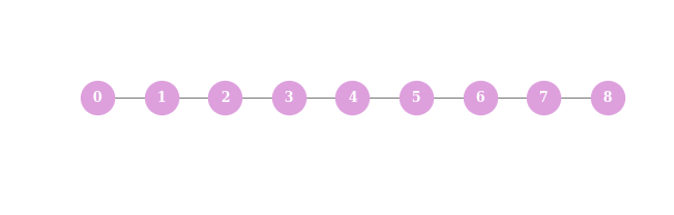
The Laplacian of such a structure looks like

L = nx.laplacian_matrix(G)

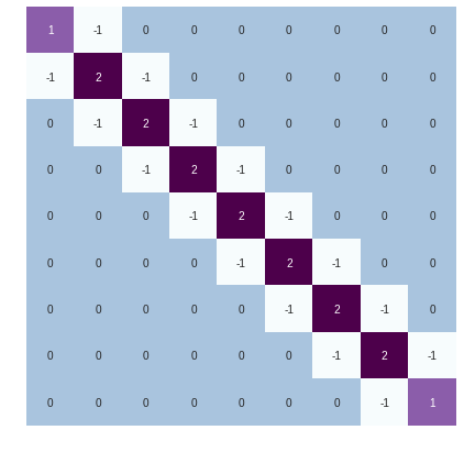
We see that the Laplacian has actually the form of the Discrete Cosine Transform (DCT), which is a variant of Fourier transform. Thus, the eigenvalues have the following analytical formulation $\chi_k:j\rightarrow\cos\Big(\big(j+\frac{1}{2}\big)\frac{k\pi}{N}\Big)$ . Next, we compare this continues formulation with the actual eigenvectors

N=9
lambd, chi = np.linalg.eigh(L.toarray())
x = np.linspace(0, N-1,100)
dct2_eigen = lambda l: np.sqrt(2/N) * np.cos(np.pi * l * (x+0.5) / N)

# abbreviated plotting code
for k, eigvec in enumerate(chi.T):
    # scaling the first eigenvector to unit $\mathbf{1}$
    if k==0:
        axes[k].plot(x, np.ones_like(x),**kw_plot_1)
        axes[k].plot(np.ones_like(eigvec), **kw_plot_2)
        axes[k].set_title("Eigen values of time-domain laplacian vs. DCT-2 eigenvalues"
                          , fontsize=16, fontname='serif')
    else:
        axes[k].plot(x, dct2_eigen(k),**kw_plot_1)
        axes[k].plot(eigvec, **kw_plot_2)
    # TODO: bug with k=6 (!?)
    if k > 5:
        break

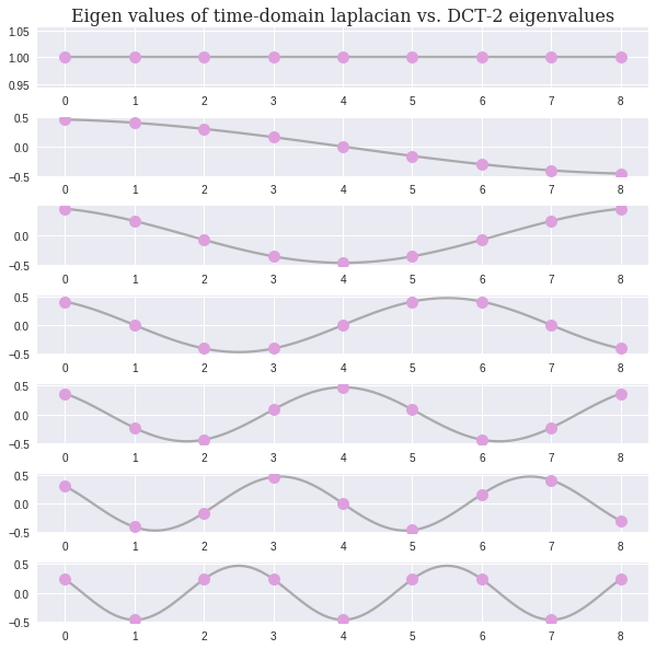
Awesome! The one dimensional Laplace operator, or the Laplacian of the time-domain graph, has the spectral representation of the Fourier Transform!

Second example - Filtering a graph signal of distance measurements

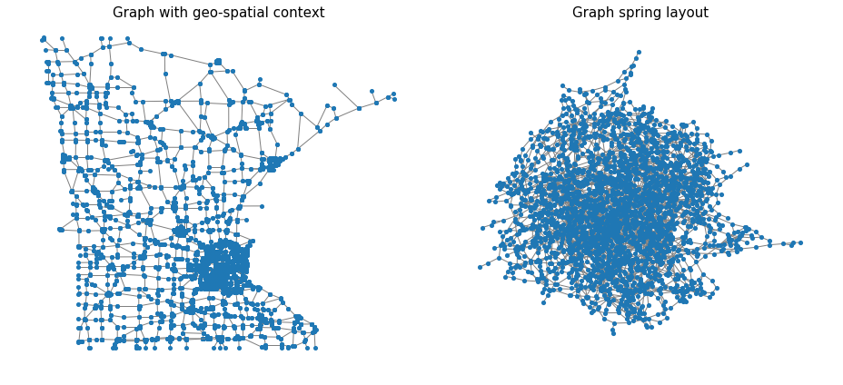
For the second example, we used the famous Minnesota road map graph. This graph holds 2642 intersections and 3304 roads. It is constructed by modeling the intersections as nodes and the roads as undirected edges. We begin by visualizing the graph with geospatial context. Every node is located according to its coordinate features. Remember, the network structure includes information only about the graph edges and is blind to the geospatial location of the node. This enables us to do very simple and visible geo-spatial manipulation, which aligns with the node’s location for a better demonstration. Here we visualize the graph with and without the geospatial context

from pygsp import graphs, filters
from pygsp import plotting
import matplotlib.pylab as plt

G = graphs.Minnesota()
G_nx = nx.Graph([tuple(r) for r in np.array(G.get_edge_list()[:2]).T]) # creating networkx graph  without geo-spatial info. This is plotted with spring layout

png

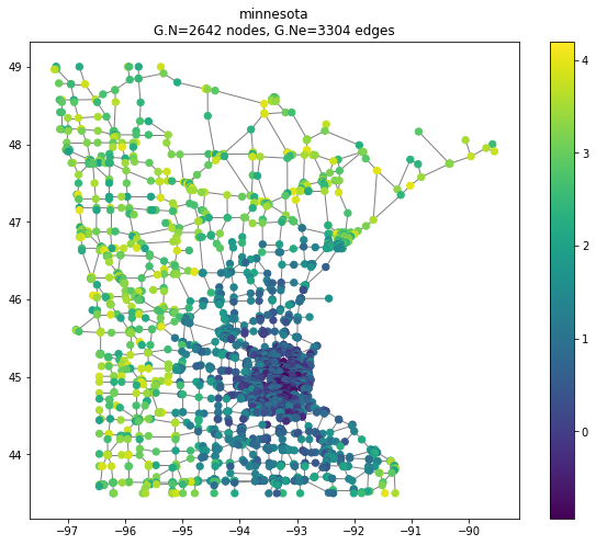
Next, we create a noisy signal based on the distance from the dense part of Minnesota, coordinates $(-93.2, 45)$ , somewhere next to Hennepin County. We added a nonlinear cutoff for $s_{in}>2$ to further localize the signal.

rs = np.random.RandomState()
s = np.zeros(G.N)
s += np.sqrt(np.sum((G.coords - np.array([-93.2, 45]))**2, axis=1))
s[s>2] = 3
s += rs.uniform(-1,1, size=G.N)

png

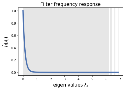
First, let’s design a heat filter and visualize it in the spectral domain. The impulse response of this filter is

$\hat{g}(x) = \exp \left( \frac{-\tau x}{\lambda_{\text{max}}} \right)$

As you can tell, this is a Low Pass filter. We choose $\tau=50$ because we want to assure the removal of higher noisy frequencies, and we assume that the spectral components that describe the clean signal have very small eigenvalues.

# First design LPF filter as a heat kernel
g = filters.Heat(G, tau=50)

png

Finally, we visualize the effect of the filter on the noisy signal

s_out = g.filter(s, method='exact') # exact uses GFT. Chebychev approx. is also available

# plotting code
fig, axes = plt.subplots(1, 2, figsize=(13, 6))
plotting.plot_signal(G, s, ax=axes[0], **plottingparam)
_ = axes[0].set_title('Noisy signal before filtering',fontsize=15)
axes[0].set_axis_off()
plotting.plot_signal(G, s_out, ax=axes[1], **plottingparam)
_ = axes[1].set_title('Filtered signal',fontsize=15)
axes[1].set_axis_off()
fig.tight_layout()
plt.show()

png

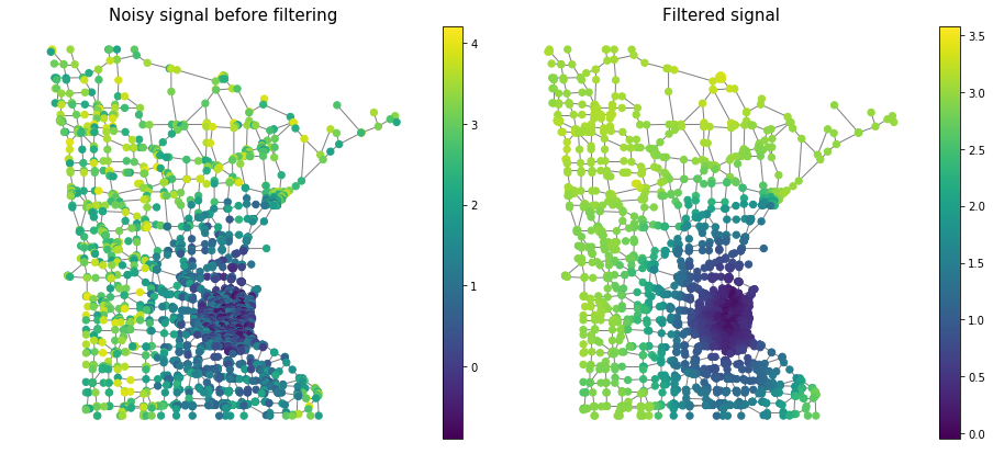
Seems like the filtering succeeded! We clearly see that the filtered signal appears to be smoother and is closer to the original noise-free distance-based signal.

Final words

That’s all for now, hope you enjoyed taking a taste from the beautiful field of GSP. I hope you now understand the relation between the spectral representation of time-domain and graph signals, and that you gained some intuition about graph frequencies in both spectral and vertex domain. Remember, this blog post is just a very basic introduction to this field.

With the resources below, you may further dive in for wavelet filter banks, spectrum-preserving graph sampling techniques, autoregressive modeling of time-graph signals or GSP applications in Big Data. Special thanks to Uriel Singer and Benny Peretz for reviewing and refining this post.